First level analysis in SPM

Specifying the Model

Since we have created the timing files previously, it is time for us to use them in conjunction with our imaging data to create statistical parametric maps. These maps could indicate that the correlation between the ideal time-series (the onset times convolved with the HRF in our model) and the time-series collected in this experiment. When we use the SPM to construct contrasts, beta weight represents the amount of modulation of the HRF, which is then transformed into a t-statistic.

To get started, create a sub-directory in sub-02 called 1stlevel so we can organize the data. Then, Open SPM GUI from Matlab terminal and select 1st-Level, select the 1stLevel directory we just created. All of the output of the 1st-level analysis will be keeped in this folder. After that, we’ll fill out the section on Timing parameters. Select Seconds for the design unit, and enter a value of 2 for Interscan Interval. Then go to Data & Design. and build three new sessions by clicking three times on New: Subject/Session. Go to the func directory and use the “Filter and Frames fields” we used before to to pick all 300 volumes of the warped usable data(file start with swar) for the first session’s Scans. And do the same for the othjer two session.

Return to the field for the first time. In the experiment, there are two conditions, and both conditions occur in each run. To construct two new condition fields, go to conditions and then New: Condition twice. Double-click on Name and type cash and explode. for the first condition.

In order to find out the onset times for each occurrence of the cash condition. From the Matlab terminal, navigate to the func directory and type:

cashRun1 = importdata(‘cash_run1.txt’); IncRun1(:,1)

Which will give you the onset times for cash condition in run_1, copy and paste the onset times onto the Onsets sector. Then we can therefore enter the number 0.772 in the Durations field, (you can check the duration time by less sub-02_task-balloonanalogrisktask_run-01_events.tsv) and SPM will assume that it is the same duration for every trial.

Repeat the process for the explode condition in run 01, as well as the cash and explode conditions in run 02 and run 03, remembering to set the duration time to 2. Here’s the code for displaying the onset times for the remaining onset times:

explodeRun1 = importdata('explode_run1.txt');
explodeRun1(:,1)

cashRun2 = importdata('cash_run2.txt');
explodeRun2(:,1)

explodeRun2 = importdata('explode_run2.txt');
explodeRun2(:,1)

cashRun3 = importdata('cash_run3.txt');
explodeRun3(:,1)

explodeRun3 = importdata('explode_run3.txt');
explodeRun3(:,1)

The names will be stored in a file called SPM.mat in the 1stLevel directory which we will look at later in more detail. Now, click the green Go button when you’re done. It should only take a few moments to estimate the model. When it’s all said and done, it should look like this:

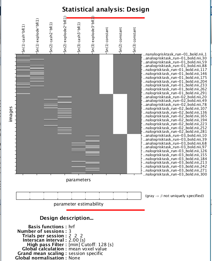
The General Linear Model for For a single subject. The ideal time-series for the cash and explode conditions for the first session are shown in the first two columns, while the ideal time-series for the conditions of run 02 are shown in the next two columns, the next two columns indicate the ideal time-series for the conditions of run 03. The last three columns are basline regressors that capture the mean signal of each run. In this figure, time runs from top to bottom, and lighter colors represent more activity.

Estimating the Model

We have created our GLM, the next step is to estimate the beta weights for each condition. Click Estimate from the SPM GUI, and select the SPM.mat from select SPM.mat tab from sub-02/1stLevel. Change the “Write residuals option” to Yes. and then click the green Go button. This will take a few minutes to run.

The Contrast Manager

When you’ve done estimating the model, it’s time to start making contrasts. what we need to do is estimate a beta weight for the cash condition and a beta weight for the explode condition. To be more specific, we can determine a contrast estimate at each voxel in the brain by take the difference betwween these two conditions. A contrast map will be generated if by doing this way.

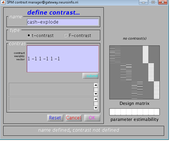
To make these contrasts, go to the Result button from SPM GUI and select the SPM.mat file that was created when the model was estimated. The design matrix is located on the right side of the screen. Select Define New Contrast and put cash-explode in the Name field.

type 1 -1 1 -1 1 -1 in the contrast vector window, then press submit. If the contrast is right, you will see “name identified, contrast defined” at the bottom of the window. Make sure your contrast manager looks like the image below, and then click OK

Examining the Output

Now, since we have set the contrast manager, click done, you will see a few options:

1 apply masking: set this to “none” becuase we want to examine all of the voxels and don’t want to restrict our analysis. 2 p value adjustment to control: Click on “none”, and set the uncorrected p-value to 0.001. This will test each voxel individually at a p-threshold of 0.01. 3 extent threshold {voxels}: Set this to 10 for now, which will only show clusters of 10 or more contiguous voxels.

We will see our results in a standardlized space in three orthogonal planes, which reflected on a glass brain once you’ve finished defining the options. The dark spots reflect clusters of voxels that passed our statistical threshold. The top-right side is a copy of our design matrix and the contrast that we are currently looking at.

The coordinates and statistical significance of each cluster are mentioned in a table at the bottom. Set-level is the first column, and it shows the likelihood of seeing the current number of clusters, c. Next, the cluster-level column shows the significance for each cluster (measured in number of voxels, or kE) using different correction methods. The “t- and z-statistics” of the peak voxel within each cluster are shown in the peak-level column, with the main clusters in bold and any sub-clusters marked in lighter front below the main cluster. Finally, in the rightmost column, the MNI coordinates of the peak for each cluster and sub-cluster are shown.The coordinates for a cluster will be highlighted in red and the cursor in the glass brain view will switch to those coordinates if you left-click on them. You can click and drag the red arrow header in the glass brain, then right-click on it and choose one of the options for jumping to the nearest suprathreshold voxel or the nearest local maximum.

From the left-button window, click on overlays/sections and then pick a standard space other than the glass brain. Go to the spm12/canonical directory and choose a brain scan such as “avg152T2”.

The results will now be shown on the template as a heatmap, The statistical table will reappear after you position the crosshairs over a specific cluster and press the “current cluster” button in the Results window, highlighting the coordinates of the cluster you picked.