Statistics and modeling

After we finish all the preprocessing steps, we can go to the next - fit a model to the data. In order to understand model fitting, we need to know 3 fundamental components:

1 General Linear Model

2 The BOLD response

3 Time-series

General linear model

The General Linear Model (GLM) is a useful framework for comparing how several variables affect the continuous variables. Although it has many variants, the simplest form is described as: Y = βX + ε. In GLM, we can use one or more regressors(X) - independent variables, to fit a model for some outcome measure(Y) - or dependent variable. To do this we need to compute numbers called beta weights(β), which are the relative weights assigned to each regressor in oder to get the best fitting for the data. Any discrepancies between the model and the data are called residuals(ε).

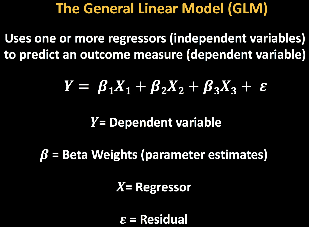
../../_images/AFNI_GLM_Equation.png — The symbols representing each of these terms are shown in the equation.

For example, imagine that we want to predict the chance of infecting Covid-19 based on social distance, daily interaction in person, and longitude. It is reasonable to find that social distanc has a negative correlation with the infection of Covid-19, the more distance you keep with other people, the less chance you will get Covid-19. In terms of daily interaction in person, it has a positive association, the more you interact with people in person, you are more likely to be affected by the virus. lastly, longitude has no associati in general.

Therefore, we need assign each of these regressors a beta weight so that the model can fit the real data best. To be more specific, maybe each additional meter for social distance is associated with an additional 0.5 decrease in infection of Covid-19, while each additional 0.5 times of personal interaction is associated with a 0.3 increase:

Chance of infecting Covid-19 (Y) = -0.5X1(social distance) + 0.3X2(personal inteaction) + ε

This GLM can be expanded to include many regressors, but no matter how many regressors you have, the GLM assumes that the data can be modeled as a linear combination of each of the regressors. Keep GLM in your mind because we will apply it in our model soon.

BOLD response

BOLD signal

In 1990, a researcher at Bell Laboratories named Seiji Ogawa discovered that more deoxygenated blood leads to a decrease in the signal measured from a brain region. An increase in oxygenated blood, on the other hand, increases the signal - this increase in oxygenated blood was later shown to be correlated with increased neural firing. This change in signal is known as blood oxygen level dependent signal ( BOLD signal). Shortly afterward, a researcher at Massachusetts General Hospital named Ken Kwong in 1992 demonstrated that the BOLD signal could be used as an indirect measure of neural activity. His experiment consisted of alternately showing a flashing checkerboard and a black screen to the subject for one minute each. The BOLD signal was recorded during each condition, as shown in the following video:

In the 1990’s, empirical studies of the BOLD signal demonstrated that, after a stimulus was presented to the subject, any part of the brain responsive to that stimulus - say, the visual cortex in response to a visual stimulus - showed an increase in BOLD signal. The BOLD signal also appeared to follow a consistent shape, peaking around six seconds and then falling back to baseline over the next several seconds. This shape can be modeled with a mathematical function called a Gamma Distribution. As Gamma Distribution is created with parameters to best fit the BOLD response observed by the these empirical studies, it is the canonical Hemodynamic Response Function(HRF).

Gamma Distribution

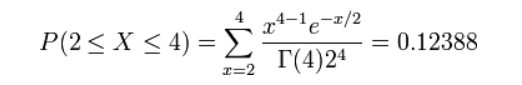
Gamma distribution is a distribution that arises naturally in processes for which the waiting times between events are relevant. It can be thought of as a waiting time between Poisson distributed events. For example, suppose you are fishing and you expect to get a fish once every 1/2 hour. Compute the probability that you will have to wait between 2 to 4 hours before you catch 4 fish.One fish every 1/2 hour means we would expect to get θ = 1 / 0.5 = 2 fish every hour on average. Using θ = 2 and k = 4, we can compute this as follows:

When applied to fMRI data, the Gamma Distribution is called a basis function because it is the fundamental element of the model we will create and fit to the time series of the data. Furthermore, if we know what the shape of the distribution looks like in response to a very brief stimulus, we can predict what it should look like in response to stimuli of varying durations, as well as any combination of stimuli presented over time.

The HRF for a Single impulse Stimulus

If the duration of a stimulus is very short, such as a snap of the fingers, we can say that it is an impulse stimulus - in other words, it has no duration. As you can see in the following figure, the shape of the BOLD signal looks like a typical Gamma Distribution, with a peak close to the beginning of the time axis (i.e., the x-axis) and a long tail to the right.

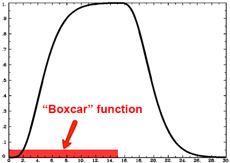
The HRF for a Single Boxcar Stimulus

Although many studies use stimuli lasting only a second or less, some studies present stimuli for longer periods of time. For example, imagine that the subject looks at a flashing checkerboard for fifteen seconds. In this case the shape of the HRF will be more spread out with a sustained peak proportional to the duration of the stimulus, falling back to baseline only after the stimulus has ended. This stimulus is called a boxcar stimulus, because it looks like a boxcar on a train.

In this case the Gamma Distribution is convolved with the boxcar stimulus. Convolution is the averaging of two functions over time; as a result, the Gamma Distribution broadens as it is averaged with the boxcar stimulus, and returns to baseline when the stimulus is removed.

Multiple HRFs overlaping

We have seen what the BOLD signal looks like after a stimulus is presented and how the HRF models the shape of that signal. But what happens if another stimulus is presented before the BOLD response for the previous stimulus has returned to baseline?

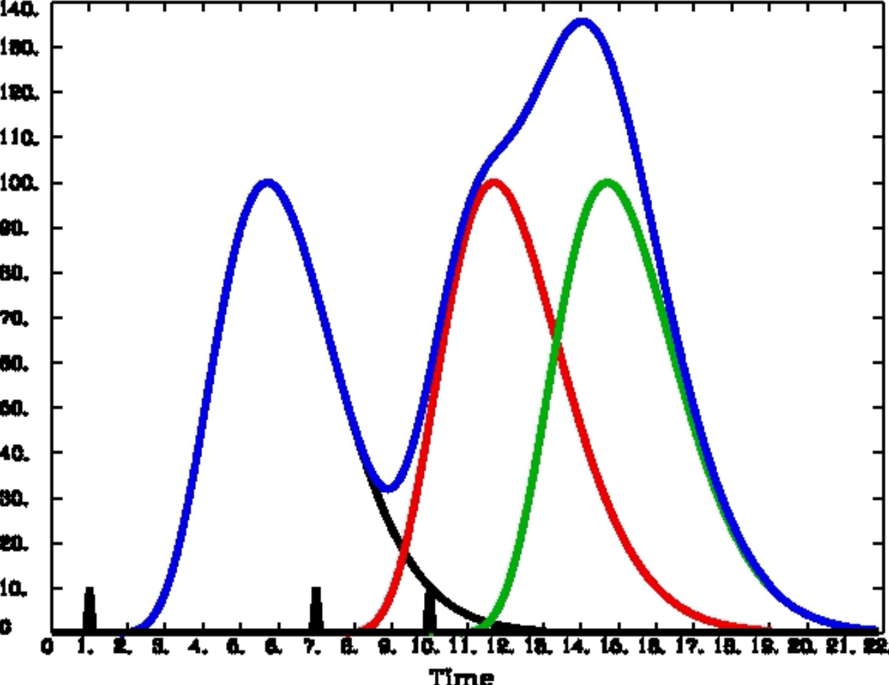
../../_images/AFNI_HRF_Sum.png — Convolution of the HRFs for individual stimuli. The overall BOLD response (blue) is a moving average of the individual HRFs outlined in black, red, and green. The vertical black lines on the x-axis represent impulse stimuli. Figure created by Bob Cox of AFNI.

In that case, the individual HRFs are summed together. This creates a BOLD response that is a moving average of the individual HRFs, and the shape of the BOLD signal becomes more complex as more stimuli are presented close together.

../../_images/AFNI_HRF_Demo.gif — Animations originally created by Bob Cox of AFNI

Time series

We have mentioned this concept several times before. As the basic composition of fMRI data. Remember that fMRI datasets contain several volumes strung together like beads on a string - we call this concatenated string of volumes a run of data. The signal that is measured at each voxel across the entire run is called a time-series. and this time-series represents the signal that is measured at each voxel during the whole scan..

Creating the time series

Since one of our goals is to create the ideal time-series so that we can use it to estimate the beta weights for our GLM, we need to create the ideal time-series first.

What do we need? Let’s take a look at the BART dataset. you could find some “event.tsv” files in the subject’s func directory. These files contain three pieces of information for the timing files. There are:

1 the experimental condition name

2 the onset time of trial for each condtion, relative to the onset of the scan

3 The duration of each trial

This information needs to be extracted from the events.tsv files and be transformed into a format that the AFNI can read. our job is to create a timing file for explode and cash experimental condition, and then split the file based on which run the condition was in. We will have 6 timing files:

1 Timings for the explode trials that occurred during the first run (explode_run1.txt)

1.2 Timings for the explode trials that occurred during the first run (explode_run2.txt)

1.3 Timings for the explode trials that occurred during the first run (explode_run3.txt)

2 Timings for the cash trials that occurred during the first run (cash_run1.txt)

2.2 Timings for the cash trials that occurred during the second run (cash_run2.txt)

2.3 Timings for the cash trials that occurred during the third run (cash_run3.txt)

Each of these timing files will have three columns:

1 Onset time, in seconds, relative to the start of the scan

2 Duration of the trial, in seconds

3 Parametric modulation(discuss later)

Next, we will condense the timing files for each run into a single file for each condition, which will be called explode.1D and cash.1D. The “1D” is a specification to AFNI; it indicates that the file contains the text information arranged in rows and columns.

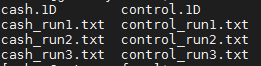
Admittedly, we will do this by our hands but not every details. There is a script that can help us to create these timing files, you can copy this can create a script in the BART directory by a text editor and name it as timing.sh, and type bash timing.sh. If evertthong goes smoothly, This will create timing files for each run for each subject on the two conditions, and save them in each subject’s func directory. You will see “cash.1D”, “control.1D” as well as “cash_run1.txt” “control_run1.txt” from “sub-02/func/:

#!/bin/bash

#Check whether the file subjList.txt exists; if not, create it
if [ ! -f subjList.txt ]; then
        ls -d sub-?? > subjList.txt
fi

#Loop over all subjects and format timing files into FSL format
for subj in `cat subjList.txt` ; do
        cd $subj/func #Navigate to the subject's func directory, which contains the timing files

        #Extract the onset times for the explode and cash trials for each run.

        cat ${subj}_task-balloonanalogrisktask_run-01_events.tsv | awk '{if ($3=="explode_demean") {print $1, $2, "1"}}' > explode_run1.txt
        cat ${subj}_task-balloonanalogrisktask_run-02_events.tsv | awk '{if ($3=="explode_demean") {print $1, $2, "1"}}' > explode_run2.txt
        cat ${subj}_task-balloonanalogrisktask_run-03_events.tsv | awk '{if ($3=="explode_demean") {print $1, $2, "1"}}' > explode_run3.txt

        cat ${subj}_task-balloonanalogrisktask_run-01_events.tsv | awk '{if ($3=="cash_demean") {print $1, $2, "1"}}' > cash_run1.txt
        cat ${subj}_task-balloonanalogrisktask_run-02_events.tsv | awk '{if ($3=="cash_demean") {print $1, $2, "1"}}' > cash_run2.txt
        cat ${subj}_task-balloonanalogrisktask_run-03_events.tsv | awk '{if ($3=="cash_demean") {print $1, $2, "1"}}' > cash_run3.txt


#Now convert to AFNI format

        timing_tool.py -fsl_timing_files explode*.txt -write_timing explode.1D

        timing_tool.py -fsl_timing_files cash*.txt -write_timing cash.1D


        cd ../..
done

Once the timing files has been created, you are now ready to use them to fit a model to the fMRI data.

Homework

In order to understand the script bettwem, you can makde some modification to extract the information for pump, control trial and make the timing files.