Preprocessing II
Slice-Timing Correction
There are no two identical wine in the world.
Most fMRI studies acquire one slice at a time, meaning that the signal recorded from one slice may be offset in time by up to several seconds when compared to another. Each of these slices takes tens to hundreds of milliseconds.The two most commonly used methods for creating volumes are sequential and interleaved slice acquisition. sequential acquisition slices have been acquired in sequential (1,2,3,4,5,6…), Interleaved slice acquisition (1,3,5,..2,4,6…) acquires every other slice and then fills in the gaps on the second pass o. Although slice timing differences may not be important for simple block design experiments, they can impact considerable errors in rapid, event-related fMRI studies if not accounted for.In addtion, the statistics model requires the time-series for each slice needs to be shifted back in time by the duration it took to acquire that slice.
Timing slice correction in AFNI
In AFNI, you could find the block of code of slice-timing correction in the proc script, it take the first slice as the reference, the code for running slice-timing correction is specified by the
-tzero 0 option of the 3dTshift command:
# ================================= tshift =================================
# time shift data so all slice timing is the same
foreach run ( $runs )
    3dTshift -tzero 0 -quintic -prefix pb01.$subj.r$run.tshift \
             pb00.$subj.r$run.tcat+orig
end
This will slice-time correct each run with the first slice as a reference. Everything in AFNI is starting from 0 in this case, the 0 in here represents the first slice of the volume. The command called
-quintic, which resamples each slice using a 5th-degree polynomial. In other words, AFNI will replace the values of the voxels within a slice by using information from a larger number of other slices.
the side effect of this method is some degree of correlation between the slices, which will be corrected later by 3dREMLfit to de-correlate the data.
Motion correction
Another influential factor for the quality is the move, even a small motion would make a difference to the wine, just like they did to the scan.
Head motion is the largest source of error in fMRI studies, If the subject in the scanner is moving, the images will look blurry.If the subject moves a lot, we also risk measuring signal from a voxel that moves. We are then in danger of measuring signal from the voxel from a different region or tissue type. It is the false positive.In addtion, motion can introduce confounds into the imaging data because motion generates signal. If the subject moves every time in response to a stimulus - for example, if he jerks his head every time he feels an electrical shock, then it can become impossible to determine whether the signal we are measuring is in response to the stimulus, or because of the movement. Therefore, a variety of strategies have been developed to cope with this problem such as immobilization of the head using padding and straps, bite bars, masks during the scanning. What’s more, the standard motion correction method of neuroimage packages considers the head as a rigid body with three directions of translation (displacement) and three axes of rotation. A single functional volume of a run is chosen as the reference to which runs in all other volumes are aligned. Procedures are performed in which each volume is rotated and aligned with the reference, with the goal to minimize a cost function. This iterative adjustment terminates once no further improvement can be achieved..
motion correction in AFNI
Motion correction in AFNI is the command 3dvolreg. In a typical analysis script generated by uber_subject.py, there will be a block of code highlighted with the header ======volreg======. There are
several commands in this block, but the most important one for our present purposes is the line that begins with “3dvolreg”:
# ================================= volreg =================================
# align each dset to base volume, align to anat, warp to tlrc space

# verify that we have a +tlrc warp dataset
if ( ! -f sub-02_T1w_ns+tlrc.HEAD ) then
    echo "** missing +tlrc warp dataset: sub-02_T1w_ns+tlrc.HEAD"
    exit
endif

# register and warp
foreach run ( $runs )
    # register each volume to the base image
    3dvolreg -verbose -zpad 1 -base vr_base_min_outlier+orig    \
             -1Dfile dfile.r$run.1D -prefix rm.epi.volreg.r$run \
             -cubic                                             \
             -1Dmatrix_save mat.r$run.vr.aff12.1D               \
             pb01.$subj.r$run.tshift+orig
You will see several options used with this command. The -base option is the reference volume; in this case, the reference image is the volume that has the lowest amount of outliers in its voxels, as
determined by an earlier command, 3dToutcount. The -1Dfile command writes the motion parameters into a text file with a “1D” appended to it, and -1Dmatrix_save saves an affine matrix which
indicates how much each TR would need to be “unwarped” along each of the affine dimensions in order to match the reference image:
# catenate volreg/epi2anat/tlrc xforms
cat_matvec -ONELINE                                         \
           sub-02_T1w_ns+tlrc::WARP_DATA -I                 \
           sub-02_T1w_al_junk_mat.aff12.1D -I               \
           mat.r$run.vr.aff12.1D > mat.r$run.warp.aff12.1D
This affine transformation matrix is then concatenated with the affine transformation matrices that were generated during the warping of the anatomical dataset to normalized space and during the alignment of the anatomical dataset to the fMRI data:
# apply catenated xform: volreg/epi2anat/tlrc 3dAllineate -base sub-02_T1w_ns+tlrc
-input pb01.$subj.r$run.tshift+orig -1Dmatrix_apply mat.r$run.warp.aff12.1D -mast_dxyz 3 -prefix rm.epi.nomask.r$run
This concatenated affine matrix is used with the 3dAllineate command to create fMRI datasets that are both motion corrected and normalized in one step (using the 1Dmatrix_apply option):
These blocks of code may be difficult to understand at first, but always keep in mind the basic structure of the AFNI commands: The command name, followed by options, and usually including a “-prefix” option to label the output. The motion correction and normalization commands often include a “-base” and “-input” pair of options as well, to indicate which dataset is being aligned to which reference dataset. You will most likely not be editing these lines of code in the file generated by uber_subject.py, but it is still useful to know why they are written the way they are; and you may use these commands outside of this script to align other datasets if you wish.
# warp the all-1 dataset for extents masking 3dAllineate -base sub-02_T1w_ns+tlrc
-input rm.epi.all1+orig -1Dmatrix_apply mat.r$run.warp.aff12.1D -mast_dxyz 3 -final NN -quiet -prefix rm.epi.1.r$run
There are some basic code structure of the AFNI commands: The command name, followed by options, and usually including a “-prefix” option to label the output. AFNI also use “-base” and “-input” pair of options to indicate which dataset is being aligned to which reference dataset. It is important for us to understand these coded since we might use these commands with different dataset individually.
Registration
The easiest and quickest way to know the quality of a wine is comparison, we need to take different wines to know which one is better and we also need a standard for a reference, we can compare each wine to each other and a standard wine for a quality assessment. So, here is the registration and normalization.
Although most people’s brains are similar - everyone has 4 lobes and subcortical, there are also differences in brain size and shape. As a consequence, if we want to do a group analysis we need to ensure that each voxel for each subject corresponds to the same part of the brain. If we are measuring a voxel in the visual cortex, make sure that every subject’s visual cortex is in alignment with each other.This alignment between the functional and anatomical images is called Registration. Most registration algorithms use the following steps:
1 Assume that the functional and anatomical images are in roughly the same location. If they are not, align the outlines of the images.
2 Take advantage of the fact that the anatomical and functional images have different contrast weightings - that is, areas where the image is dark on the anatomical image (such as cerebrospinal fluid) will appear bright on the functional image, and vice versa. This is called mutual information. The registration algorithm moves the images around to test different overlays of the anatomical and functional images, matching the bright voxels on one image with the dark voxels of another image, and the dark with the bright, until it finds a match that cannot be improved upon.
3 Once the best match has been found, then the same transformations that were used to warp the anatomical image to the template are applied to the functional images.
Registration with AFNI
The command align_epi_anat.py can do several preprocessing steps at once - registration, aligning the volumes of the functional images together, and slice-timing correction. In here, we will just use
it for registration. The code for this step will be found in proc.sub_02 script:
# ================================= align ==================================
# for e2a: compute anat alignment transformation to EPI registration base
# (new anat will be intermediate, stripped, sub-02_T1w_ns+orig)
align_epi_anat.py -anat2epi -anat sub-02_T1w+orig \
       -save_skullstrip -suffix _al_junk          \
       -epi vr_base_min_outlier+orig -epi_base 0  \
       -epi_strip 3dAutomask                      \
       -cost lpc+ZZ -giant_move                   \
       -volreg off -tshift off
We will introduce these different options in more details:
1 -anat2epi : will align anatomical to EPI dataset, which is the default setting in AFNI.
2 -anat: use anatomical dataset to align or to which to align.
3 save_skullstrip : save skull-stripped (not aligned).
4 -suffix with the string “_al_junk” to some of the intermediate stages of the registration, and for normalization later.
5 -epi_base : the epi base used in alignment, The “epi” options signalize that the functional volume with the least variability will be used as a reference image, and non-brain tissue is stripped by
3dAutomask , an alternative to 3dSkullStrip.
7 lpc (Localized Pearson Correlation) function. The ‘lpc’ cost function is computed by the 3dAllineate program.
8 -giant_move attempts to find a good initial starting alignment between the anatomical and functional images, giant_move option will usually work well too,but it adds significant time to the
processing and allows for the possibility of a very bad alignment.
9 The last two options -volreg off, -tshift off indicate that we do not want to include alignment and slice-timing correction in the current command.
Normalization
Each brain needs to be transformed to have the same size, shape, and dimensions to be compared. We do this by normalizing (or warping) to a template. A template is a brain that has standard dimensions and coordinates, Each subjects’ functional images will be transformed to match the general shape and large anatomical features of the template. Most researchers have agreed to use them when reporting their results.The dimensions and coordinates of the template brain are also referred to as standardized space.
Normalization with AFNI’s @auto_tlrc
Once we have aligned the anatomical and functional images, the next step for us is to normalize the anatomical image to a template as well as functional image. We will use the @auto_tlrc command to do
this.To normalize the anatomical image,; this and a following command, cat_matvec, are found in your proc script:
# ================================== tlrc ==================================
# warp anatomy to standard space
@auto_tlrc -base MNI_avg152T1+tlrc -input sub-02_T1w_ns+orig -no_ss

# store forward transformation matrix in a text file
cat_matvec sub-02_T1w_ns+tlrc::WARP_DATA -I > warp.anat.Xat.1D
The first block of commands indicates that we take the image MNI_avg152T1 as a template, and the skull-stripped anatomical image as a source image. The -no_ss option indicates that the anatomical
image has already been skull-stripped. The anatomical image needs to be moved and transformed so that it can align the template and the anatomical image. The second command, cat_matvec, extracts this
matrix and copies it into a file called warp.anat.Xat.1D.
Smoothing
If we have the best wine, why don’t to mix it with other drinks in order to achieve the best taste? It is common for neuroimage software to smooth the functional data, or replace the signal at each voxel with a weighted average of that voxel’s neighbors. This may seem strange at first - why would we want to make the images blurrier than they already are?
Spatial smoothing is the averaging of signals from adjacent voxels. This improves the signal-to-noise ratio (SNR) but decreases spatial resolution, blurs the image, and smears activated areas into adjacent voxels. The process can be justified because closely neighboring brain voxels are usually inherently correlated in their function and blood supply. The standard method is to convolve (“multiply”) the fMRI data with a 3D Gaussian kernel (“filter”) that averages signals from neighboring voxels with weights that decrease with increasing distance from the target voxel. In practice, the full width half maximum (FWHM) value of the Gaussian spatial filter is typically set to about 4-6 mm for single subject studies and to about 6-8 mm for multi-subject analyses. The benefits of smoothing can outweigh the drawbacks:
1 We know that fMRI data contain a lot of noise, and that the noise is frequently greater than the signal. By averaging over nearby voxels we can cancel out the noise and enhance the signal.
2 Smoothing can be good for group analyses in which all of the subjects’ images have been normalized to a template. If the images are smoothed, there will be more overlap between clusters of signal, and therefore greater likelihood of detecting a significant effect. ``3dmerge``in AFNI will do smoothing for us, you will find further details in proc script:
# ================================== blur ==================================
# blur each volume of each run
foreach run ( $runs )
    3dmerge -1blur_fwhm 4.0 -doall -prefix pb03.$subj.r$run.blur \
            pb02.$subj.r$run.volreg+tlrc
end
The -1blur_fwhm specifies the amount to smooth the image in 4mm. -doall applies this smoothing kernel to each volume in the image, and the -prefix option, we you might know, specifies the name of the output dataset.
Masking
The last preprocessing steps will take these smoothed images and then scale them to have a mean signal intensity of 100 - so that deviations from the mean can be measured in percent signal change. Any non-brain voxels will then be removed by a mask, and these images will be ready for statistical analysis.
As you might see before, a volume of fMRI data includes both the areas that we are interested in and the irrevelant regions such as the brain and the surrounding skull, neck and ear. And we have large numbers of voxels that comprise the air outside the head.we can create a mask for our data to reduce the irrelevant regions of our datasets and speed up our analyses, A mask simply tells the programer which voxels are worth to be analyzed - any voxels within the mask have their original values, or can be assigned a value of 1, whereas any voxels outside mask are assigned a value of zero. Anything outside the mask will be assumed as noise.
Masks are created with 3dAutomask command, which requires arguments for input and output datasets:
# ================================== mask ==================================
# create 'full_mask' dataset (union mask)
foreach run ( $runs )
    3dAutomask -dilate 1 -prefix rm.mask_r$run pb03.$subj.r$run.blur+tlrc
end
-dilate 1 means AFNI will dilate the mask outwards ‘1’ times:
# create union of inputs, output type is byte
3dmask_tool -inputs rm.mask_r*+tlrc.HEAD -union -prefix full_mask.$subj

# ---- create subject anatomy mask, mask_anat.$subj+tlrc ----
#      (resampled from tlrc anat)
3dresample -master full_mask.$subj+tlrc -input sub-02_T1w_ns+tlrc     \
         -prefix rm.resam.anat

# convert to binary anat mask; fill gaps and holes
3dmask_tool -dilate_input 5 -5 -fill_holes -input rm.resam.anat+tlrc  \
            -prefix mask_anat.$subj

# compute tighter EPI mask by intersecting with anat mask
3dmask_tool -input full_mask.$subj+tlrc mask_anat.$subj+tlrc          \
            -inter -prefix mask_epi_anat.$subj

# compute overlaps between anat and EPI masks
3dABoverlap -no_automask full_mask.$subj+tlrc mask_anat.$subj+tlrc    \
            |& tee out.mask_ae_overlap.txt

# note Dice coefficient of masks, as well
3ddot -dodice full_mask.$subj+tlrc mask_anat.$subj+tlrc               \
      |& tee out.mask_ae_dice.txt

# ---- create group anatomy mask, mask_group+tlrc ----
#      (resampled from tlrc base anat, MNI_avg152T1+tlrc)
3dresample -master full_mask.$subj+tlrc -prefix ./rm.resam.group      \
           -input /opt/afni/MNI_avg152T1+tlrc

# convert to binary group mask; fill gaps and holes
3dmask_tool -dilate_input 5 -5 -fill_holes -input rm.resam.group+tlrc \
            -prefix mask_group
The rest of the code within the “mask” block creates a union of masks that represents the extent of all of the individual fMRI datasets in the experiment. It then computes a mask for the anatomical dataset, and then takes the intersection of the fMRI and anatomical masks
Scaling
One problem with fMRI data is that we collect data with units that are arbitrary, and of themselves meaningless. The intensity of the signal that we collect can vary from run to run, and from subject to subject. The only way to create a useful comparison within or between subjects is to take the contrast of the signal intensity between conditions, as represented by a beta weight (which will be discussed later in the chapter on statistics).
In order to make the comparison of signal intensity meaningful between studies as well, AFNI scales the timeseries in each voxel individually to a mean of 100:
# ================================= scale ==================================
# scale each voxel time series to have a mean of 100
# (be sure no negatives creep in)
# (subject to a range of [0,200])
foreach run ( $runs )
    3dTstat -prefix rm.mean_r$run pb03.$subj.r$run.blur+tlrc
    3dcalc -a pb03.$subj.r$run.blur+tlrc -b rm.mean_r$run+tlrc \
           -c mask_epi_extents+tlrc                            \
           -expr 'c * min(200, a/b*100)*step(a)*step(b)'       \
           -prefix pb04.$subj.r$run.scale
end
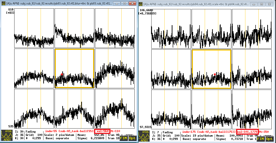
You can see these changes in the time-series graph below. Note that the values in the first image are relatively high - in the 600s - and that they are arbitrary; they could just as easily be around 500 or 900 in another subject. By scaling each subject’s data to the same mean, as in the right image, we can place each run of each subject’s data on the same scale to compare.