4 Lay of the land: medial temporal lobes landmarks

With your segmentation notes spreadsheet open in a separate window, start by identifying the landmarks outlined in the following section. This process will allow you to get a “feel” for your particular subject’s anatomy before you actually start segmenting. You will make notes about these landmarks and which slice you identify them in your spreadsheet. It is recommended that you move in an anterior-posterior direction when identifying these landmarks. It is critical that you follow the order outlined in this section, as certain earlier decisions on landmarks will inform later ones. Screenshots with examples are included to help you. Please note, however, that you will need to read the rules for each landmark carefully as your T2 images will certainly vary greatly (see Variability in Landmarks for more information).

LANDMARK 1: FIRST SLICE CONTAINING THE COLLATERAL SULCUS

The first slice of the MTL is the first slice in your image set where you can clearly see grey matter ribbon only consists of the perirhinal cortex. The depth of the CS determines is important to identify the CS first. In your spreadsheet, note down the first and most anter example below.

Figure 4.1: The first appearance of the collateral sulcus (CS) in a T2-weighted MR image.

Be careful - in some brains it is easy to confuse a prominent rhinal sulcus (RS) with the Sulcus in Segmenting Regions of Interest in the Medial Temporal Lobes**

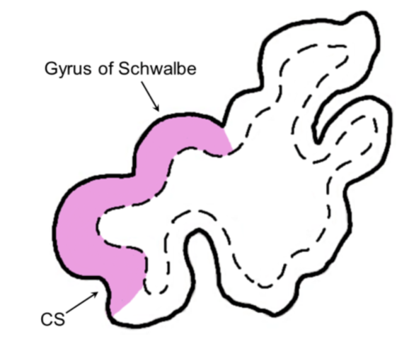
Figure 4.2: According to Insausti et al. (1998), the first appearance of the CS marks the transition between the temporopolar cortex (not included in the OAP protocol) and the perirhinal cortex (shown here in pink). Image adapted from Insausti et al. (1998). CS = collateral sulcus

LANDMARK 2: THE FRONTAL-TEMPORAL JUNCTION/LIMEN INSULAE.

This key landmark will determine where you start drawing the entorhinal cortex (ERC). To find this landmark, look for the frontal-temporal junction (FTJ)/limen insulae. The slice in which there is a clear band of white matter that joins the frontal lobe to the temporal lobe is the slice in which the FTJ/limen insulae is indicated. It is sometimes easier to visualize this landmark on a T1-weighted scan.

Figure 4.3: The two examples here compare a slice (T2-weighted) in which the limen insulae grey matter is visible in the left image; however, there is no clear white matter connection between the temporal and frontal lobe yet, versus in right image there is a clear connection between the white matter of the frontal and temporal lobe. This is a clear indication of the presence of the FTJ/limen insula, which will determine the delineation of the entorhinal cortex. See the next image below for another example.

Figure 4.4: Adapted from Insausti et al. (1998). (A) The emergence of CS and gyrus of Schwalbe (with PRC depicted in pink), (B) Moving posteriorly, the limen insula is now present but the white matter connection between the frontal and temporal lobe is not clear, so we only continue to trace the PRC. (C) There is a clear connection between the white matter of the frontal lobe and temporal lobe. This is the slice in which you draw the ERC (depicted in blue) from the PRC up to the uncal notch (un). This is also the slice in which you make a note in your spreadsheet for the presence of the FTJ/limen insula. Boundaries based on Kivisaari et al. (2013), see Helpful Additional Resources for Further Reading.

Figure 4.5: This image brings together the first two landmarks (CS and FTJ/limen insulae) as described above. As you move from anterior to posterior, the CS may change from a single to double CS.

LANDMARK 3: THE FIRST SLICE CONTAINING VISIBLE HIPPOCAMPAL HEAD

Next, you will need to look for the hippocampal head. To find this landmark:

A In its first appearance, the hippocampal head will probably look like a “bean” shape
B The amygdala is located superior and the ventricle is lateral to the hippocampal head
C Ambient gyrus appears in the same slice as the appearance of the hippocampal head

Figure 4.6: This image depicts the first appearance of the hippocampal head (shown in orange). Notice the ventricle laterally, and the ambient gyrus medially.

Figure 4.7: This image will help you determine the shape of the hippocampal head in the brain you are segmenting. The example shown is adapted from Ding et al. (2015). Notice how the head shape can resemble a “bean” (A1, A2, B1, B2) or more like the hippocampal body (C1, C2).

LANDMARK 4: THE FIRST SLICE CONTAINING DENTATE GYRUS

After identifying the hippocampal head on 2-3 slices (depending on the brain you are segmenting and the quality of the T2 scan) you will start to see subfields of the hippocampus. At this point, the hippocampus will look thicker than previous slices and the superior digitations of the hippocampus will have smoothed out. This is the first slice of the dentate gyrus (DG) and, by extension, other subfields of the hippocampus. Finally, a darker C-shaped band should be visible, separating hippocampal cornu ammonis area 1 (CA1) from DG. Note that in the OAP protocol, we do not distinguish between DG and cornu ammonis area 3 (CA3).

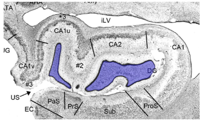
Figure 4.8: The image above, adapted from Ding et al. (2015), will help you with identifying dentate gyrus (highlighted in blue).

LANDMARK 5: THE LAST SLICE CONTAINING THE UNCUS

The last slice of the uncus in the image below would be the second box from the left. You should note here that this EC/PRC to PHC transition is valid for 2-3mm thick slices. For thinner slices, there will be more slices in between the uncal apex and the start of the PHC (Pruessner et al. (2000) suggests it starts 5mm posterior to the uncal apex).

Figure 4.9: Anterior to posterior cortical transition showing the final slice containing the uncus. After one slice where the uncus is absent, you can start tracing the PHC, and the ERC/PRC disappears. Image adapted from: Carr, V.A. (2013), Variability in collateral sulcus anatomy: The challenge of reliably segmenting medial temporal lobe cortices. Hippocampal Subfield Segmentation Summit, Davis: Oral presentation.

LANDMARK 6: THE LAST APPEARANCE OF THE COLLICULI

The last clear appearance of the colliculi is the final slice where we segment the hippocampal subfields. After this slice, the hippocampus transitions to the tail segment.

Figure 4.10: The final appearance of the colliculi, which resemble a “butterfly” shape in the centre of the brain.

Figure 4.11: On the left, the final posterior slice of the hippocampal body, containing the colliculi, crus fornix, and the “tear drop” shape of the hippocampal body. On the right, the colliculi are no longer visible, making the first slice of the hippocampal tail.

LANDMARK 7: THE LAST SLICE WHERE THE HIPPOCAMPAL TAIL IS VISIBLE

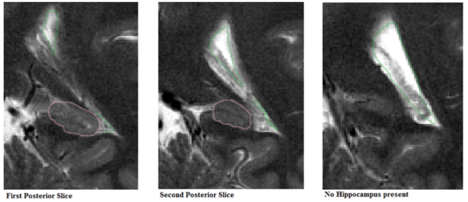
Figure 4.12: The “sweeping” of CSF towards the superior ventricle means that the hippocampal tail is no longer present in posterior slices.

The last slice of the MTL is the slice in your image set where you can clearly see the grey matter portion of the hippocampus tail. After the last slice of the MTL the bright CSF laterally to the hippocampus will clearly sweep up and meet up with the more superior ventricle.