3rd level analysis
One of the goals in the fMRI analysis is to generalize the results of the sample to the population. If we see changes in brain activity in the sample, how can we ensure that these changes would likely be seen in the population? To answer that question, a 3rd-level analysis, group-level analysis, is needed. we need to calculate the standard error and the mean for a contrast estimate, and then test whether the average estimate is statistically significant.
FSL can only run one model at a time. In this example, we will run a 3rd-level analysis for the contrast of explode-cash (it is cope3 from the 2nd-level analysis because it was the third contrast
that was specified).
Loading the Data
From the BART directory, open the FEAT GUI. As we did in the 2nd-level analysis, select Higher-level analysis, instead of input are lower-level FEAT directories, choose Inputs are 3D cope images
from FEAT directories, and change the number of inputs to 16. Since the 2nd-level analysis generated an average contrast of parameter estimate (cope) for each subject for each contrast that was
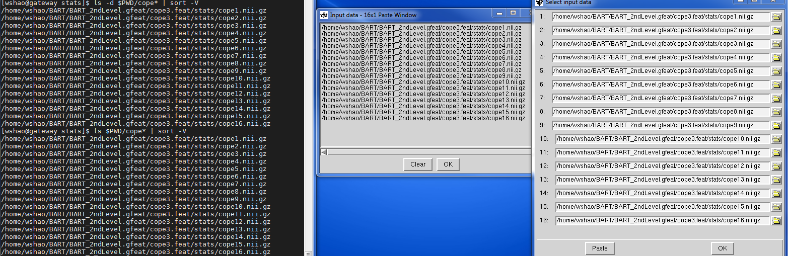
specified in our model. Regarding selecting the FEAT directories, we can copy and paste a list of the cope images: Click on Select cope images and then click the Paste button. In a new Terminal, navigate
to the directory BART_2ndLevel.gfeat/cope3.feat/stats, and type ls $PWD/cope* | sort -V. This will list all of the cope images in numerical order, copy and paste the list into the Input data
dashboard window by typing Ctrl+c and ctrl+y. After clicking OK, label the output directory BART_3rdLevel_explode-cash.
Creating the GLM
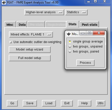
Move to the Stats tab. For a 3rd-level analysis, we will use the Mixed Effects FlAME 1. This model assigns weight based on the variance to ensure that our results of the sample are generalizable to the population our sample was drawn from. It provides accurate parameter estimates by using information about both within-subject and between-subject variability.
Due to the simple design, we can quickly create a GLM by using the Model setup wizard. as we have already taken the contrast for each subject, single group average would be a good choice. When you
click Process, you should see a Model representation that looks like this:
The Post-Stats Tab
Now we finally could discuss the Post-Stats tab. we only care about in here the Thresholding options:
1 None won’t do any thresholding (i.e., show the parameter estimate at every voxel, regardless of significance)
2 Uncorrected will allow any individual voxels to pass the threshold specified in Z-threshold (e.g., here we would only show voxels that have a value greater than 3.1);
3 Voxel will perform a type of maximum height thresholding based on Gaussian Random Field theory, which is less conservative than a Bonferroni test
4 Cluster, which uses a cluster-defining threshold (CDT) to determine whether a cluster of voxels is significant. The logic behind this approach is that neighboring voxels are not independent of one another, and this reduced degrees of freedom is taken into account when estimating significance.
For example, if we leave our Z-threshold at 3.1 and our Cluster p-threshold at 0.05, we will look for clusters composed of voxels that each individually pass a z-threshold of 3.1. FSL runs simulations to see how often we would get clusters of certain sizes with each of their constituent voxels passing that z-threshold, and creates a distribution of cluster sizes for that CDT. Cluster sizes that occur less than 5% of the time in the simulations for that CDT are then determined to be significant.
The default of a Cluster correction setting for most analysis is that z=3.1 and a cluster threshold of p=0.05, which is reasonable unless you have a good reason to change it. Now click Go. This
process will take about 5-10 minutes, depending on how powerful your computer is.
Reviewing the Output
In the FEAT HTML output, you will see the thresholded z-statistic image overlaid on a template MNI brain. These are axial slices, and they give you a quick overview of where the significant clusters are located.


As you can see, I have run two tests with z = 1 and 2.3. as you can see, the results will change according to the z score.
In order to take a closer look at the results, open fslview and load a standard template, such as MNI152_T1_2mm_brain. Then load the thresh_zstat1.nii.gz image, located in
BART_3rdLevel_explode-cash.gfeat/cope3.feat. This image only shows those clusters that were determined to be significant based on the criteria you specified in the Post-stats tab. Change the color scheme
to “Red-Yellow”, and change the “Min.” value to 3.1. You can also click on the Gear icon and change the interpolation to make the results look smoother. Lastly, click on a cluster in the dorsal medial
prefrontal cortex area, and turn the crossha Cirs off by clicking on the crosshairs icon. You can then take a snapshot of this montage with the Camera icon, and include the image as a figure in your
manuscript.