Running GLM on python

Since we have the basic knowledge of the tool. Let’s start the fun with running fMRI analysis code on python.

HCP dataset and Gamblining project

HCP

The Human Connectome Project (HCP) is a data sharing initiative to address fundamental questions about human anatomy and variation related to neuron connectivity. It is based at Washington University and includes collaborations between University of Southern California, Harvard and Massachusetts General Hospital.The HCP collected scanned the brains of more than 1200 young men and women, mostly in their 20s, participants also completed questionnaires about their health and lives, an aerobic fitness walking test and cognitive tests.

The HCP dataset comprises task-based fMRI from a large sample of human subjects. The dataset includes time series data that has been preprocessed and spatially-downsampled by aggregating within 360 regions of interest. In order to use this dataset, please electronically sign the HCP data use terms at ConnectomeDB. Although We are only use the gambling sub dataset for this chapter, you can apply the code with different dataset once you learned the code.

Instructions for this dataset are on pp. 24-25,36 and 50-51 of the HcP Reference Manual. you are more than welcome to study this manual before the analysis

Gambling project

This task was adapted from the one developed by Delgado and Fiez (Delgado et al. 2000). Participants play a card guessing game where they are asked to guess the number on a mystery card (represented by a “?”) in order to win or lose money. Participants are told that potential card numbers range from 1-9 and to indicate if they think the mystery card number is more or less than 5 by pressing one of two buttons on the response box. Feedback is the number on the card (generated by the program as a function of whether the trial was a reward, loss or neutral trial) and either: 1) a green up arrow with “$1” for reward trials, 2) a red down arrow next to -$0.50 for loss trials; or 3) the number 5 and a gray double headed arrow for neutral trials. The “?” is presented for up to 1500 ms (if the participant responds before 1500 ms, a fixation cross is displayed for the remaining time), following by feedback for 1000 ms. There is a 1000 ms with a “+” presented on the screen. The task is presented in blocks of 8 trials that are either mostly reward (6 reward trials pseudo randomly interleaved with either 1 neutral and 1 loss trial, 2 neutral trials, or 2 loss trials) or mostly loss (6 loss trials pseudorandomly interleaved with either 1 neutral and 1 reward trial, 2 neutral trials, or 2 reward trials). In each of the two runs, there are 2 mostly reward and 2 mostly loss blocks, interleaved with 4 fixation blocks (15 seconds each).

Some Credits of this chapter go to Neuromatch Academy.

Running the analysis

Now, let’s open the VSC and the jupyter book. You also can see and run all the code from Colaboratory here. each of them has its own advantage, depending on your preference.

Once you are familiar with the dataset, we can start by loading the libraries:

import os
import numpy as np
import matplotlib.pyplot as plt
import nibabel as nib
import pandas as pd
import seaborn as sns
from sklearn.linear_model import LogisticRegression
from sklearn.model_selection import cross_val_score

Next, let’s setting the figure for the visualization:

#title Figure settings

%matplotlib inline

%config InlineBackend.figure_format = 'retina'

plt.style.use("https://raw.githubusercontent.com/NeuromatchAcademy/course-content/master/nma.mplstyle")

Once we set up the figure, set up with data and environment would be the next:

# The download cells will store the data in nested directories starting here:
HCP_DIR = "./hcp"
if not os.path.isdir(HCP_DIR):
os.mkdir(HCP_DIR)

# The data shared for NMA projects is a subset of the full HCP dataset
N_SUBJECTS = 339

# The data have already been aggregated into ROIs from the Glasser parcellation
N_PARCELS = 360

# The acquisition parameters for all tasks were identical
TR = 0.72  # Time resolution, in seconds

# The parcels are matched across hemispheres with the same order
HEMIS = ["Right", "Left"]

# Each experiment was repeated twice in each subject
N_RUNS = 2

# There are 7 tasks in the dataset. Each has a number of 'conditions'. and we are only use the gambling data

EXPERIMENTS = {
    'GAMBLING'   : {'runs': [11,12], 'cond':['loss','win','neut']}
}

# Load all subjects all subjects:
subjects = range(N_SUBJECTS)

For more information about the files in the gambling project, go 45-47 page of HCP Reference Manual.

Download the data, the task data are shared in different files, but we will unpack them into the same directory structure:

fname = "hcp_task.tgz"
if not os.path.exists(fname):
!wget -qO $fname https://osf.io/s4h8j/download/
!tar -xzf $fname -C $HCP_DIR --strip-components=1

Loading region information.Downloading this dataset will create the regions.npy file, which contains the region name and network assignment for each parcel:

regions = np.load(f"{HCP_DIR}/regions.npy").T
region_info = dict(
   name=regions[0].tolist(),
   network=regions[1],
   hemi=['Right']*int(N_PARCELS/2) + ['Left']*int(N_PARCELS/2),
)

Loading the time series from a single suject and a single run, and one for loading an EV file for each task.An EV file (EV:Explanatory Variable) describes the task experiment in terms of stimulus onset, duration, and amplitude. These can be used to model the task time series data:

def load_single_timeseries(subject, experiment, run, remove_mean=True):
#Load timeseries data for a single subject and single run.

Args:
  subject (int):      0-based subject ID to load
  experiment (str):   Name of experiment
  run (int):          0-based run index, across all tasks
  remove_mean (bool): If True, subtract the parcel-wise mean (typically the mean BOLD signal is not of interest)

Returns
  ts (n_parcel x n_timepoint array): Array of BOLD data values

bold_run  = EXPERIMENTS[experiment]['runs'][run]
bold_path = f"{HCP_DIR}/subjects/{subject}/timeseries"
bold_file = f"bold{bold_run}_Atlas_MSMAll_Glasser360Cortical.npy"
ts = np.load(f"{bold_path}/{bold_file}")
if remove_mean:
  ts -= ts.mean(axis=1, keepdims=True)
return ts


def load_evs(subject, experiment, run):
#Load EVs (explanatory variables) data for one task experiment.

Args:
  subject (int): 0-based subject ID to load
  experiment (str) : Name of experiment

Returns
  evs (list of lists): A list of frames associated with each condition

frames_list = []
task_key = 'tfMRI_'+experiment+'_'+['RL','LR'][run]
for cond in EXPERIMENTS[experiment]['cond']:
  ev_file  = f"{HCP_DIR}/subjects/{subject}/EVs/{task_key}/{cond}.txt"
  ev_array = np.loadtxt(ev_file, ndmin=2, unpack=True)
  ev       = dict(zip(["onset", "duration", "amplitude"], ev_array))
  # Determine when trial starts, rounded down
  start = np.floor(ev["onset"] / TR).astype(int)
  # Use trial duration to determine how many frames to include for trial
  duration = np.ceil(ev["duration"] / TR).astype(int)
  # Take the range of frames that correspond to this specific trial
  frames = [s + np.arange(0, d) for s, d in zip(start, duration)]
  frames_list.append(frames)

return frames_list

OK, let’s load the timeseries data for the GAMBLING experiment from a single subject and a single run:

my_exp  = 'GAMBLING'
my_subj = 0
my_run  = 1
data = load_single_timeseries(subject=my_subj,experiment=my_exp,run=my_run,remove_mean=True)
#print the data shape
print(data.shape)

As you can see the time series data contains 284 time points in 360 regions of interest (ROIs).Now in order to understand how to model these data, we need to relate the time series to the experimental manipulation. This is described by the EV files. Let us load the EVs for this experiment:

evs = load_evs(subject=my_subj, experiment=my_exp,run=my_run)
# lets visualzie the loss regressor
los_reg = np.zeros(253)
win_reg = np.zeros(253)
net_reg = np.zeros(253)
res_reg = np.ones(253)

for id in range(0,len(evs[0])):
    los_reg[evs[0][id]] = 1
# lets visualize the win regressor
for id in range(0,len(evs[1])):
    win_reg[evs[1][id]] = 1
# lets visualize the neut regressor
for id in range(0,len(evs[2])):
    net_reg[evs[2][id]] = 1
#let screate the resting phase regressor
for id in range(0,len(evs[0])):
    res_reg[evs[0][id]] = 0
for id in range(0,len(evs[1])):
    res_reg[evs[1][id]] = 0
for id in range(0,len(evs[2])):
    res_reg[evs[2][id]] = 0

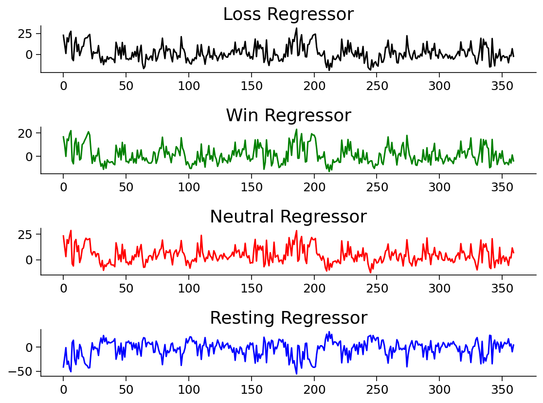
Let’s take a look at the regressor:

fig, axs = plt.subplots(2,2, figsize=[15, 6])
axs[0,0].plot(los_reg, 'k')
axs[0, 0].set_title('Loss Regressor')
axs[0,1].plot(win_reg, 'g')
axs[0, 1].set_title('Win Regressor')
axs[1,0].plot(net_reg, 'r')
axs[1, 0].set_title('Neutral Regressor')
axs[1,1].plot(res_reg, 'b')
axs[1, 1].set_title('Resting Regressor')

Next, one of the most important functions in fMRI, general linear model:

def glm(data,reg):
    constant = np.ones(253)
    X = np.vstack((reg, constant)).T
    y = data

    # Calculate the dot product of the transposed design matrix and the design matrix
    # and invert the resulting matrix.
    tmp   = np.linalg.inv(X.transpose().dot(X))

    # Now calculate the dot product of the above result and the transposed design matrix
    tmp   = tmp.dot(X.transpose())

    # Pre-allocate variables
    beta  = np.zeros((y.shape[0], X.shape[1]))
    e     = np.zeros(y.shape)
    model = np.zeros(y.shape)
    r     = np.zeros(y.shape[0])

# Find beta values for each voxel and calculate the model, error and the correlation coefficients
    for i in range(y.shape[0]):
        beta[i]  = tmp.dot(y[i,:].transpose())
        model[i] = X.dot(beta[i])
        e[i]     = (y[i,:] - model[i])
        r[i]     = np.sqrt(model[i].var()/y[i,:].var())


    return beta, model, e, r

OK, now, let’s apply the function into our data for one example:

X = np.vstack((los_reg, win_reg, net_reg, res_reg)).T
y = data
constant = np.ones(253)
c = np.vstack(constant)

# Calculate the dot product of the transposed design matrix and the design matrix
# and invert the resulting matrix.

tmp   = np.linalg.inv(X.transpose().dot(X))

# Now calculate the dot product of the above result and the transposed design matrix

tmp   = tmp.dot(X.transpose())

# Pre-allocate variables
beta  = np.zeros((y.shape[0], X.shape[1]))
e     = np.zeros(y.shape)
model = np.zeros(y.shape)
r     = np.zeros(y.shape[0])

So far so good, let’s apply the model for all the subjects, all runs and all condition:

# Lets bring together the previous steps all in one for running through all subjects, all runs
# Create the beta for 4 conditions
betas_los = np.zeros((2, 360, 2, 339))
betas_win = np.zeros((2, 360, 2, 339))
betas_net = np.zeros((2, 360, 2, 339))
betas_res = np.zeros((2, 360, 2, 339))

# Create R for 4 conditions
r_los = np.zeros((1,360,2,339))
r_win = np.zeros((1,360,2,339))
r_net = np.zeros((1,360,2,339))
r_res = np.zeros((1,360,2,339))
for sub_id in subjects:
    my_exp  = 'GAMBLING'
    my_subj = sub_id
    for run in [0,1]:
        my_run  = run
        #load data
        data = load_single_timeseries(subject=my_subj,experiment=my_exp,run=my_run,remove_mean=True)
        # load the evs and create regressors
        evs = load_evs(subject=my_subj, experiment=my_exp,run=my_run)
        los_reg = np.zeros(253)
        win_reg = np.zeros(253)
        net_reg = np.zeros(253)
        res_reg = np.ones(253)
        #visualzie the loss regressor
        for id in range(0,len(evs[0])): los_reg[evs[0][id]] = 1
        # lets visualize the win regressor
        for id in range(0,len(evs[1])): win_reg[evs[1][id]] = 1
        # lets visualize the neutral regressor
        for id in range(0,len(evs[2])): net_reg[evs[2][id]] = 1
        #let create the resting phase regressor
        for id in range(0,len(evs[0])): res_reg[evs[0][id]] = 0
        for id in range(0,len(evs[1])): res_reg[evs[1][id]] = 0
        for id in range(0,len(evs[2])): res_reg[evs[2][id]] = 0
        #let create the model structure for all
        betas_los_tmp, model_los_tmp, e_los_tmp, r_los_tmp = glm(data, los_reg)
        betas_win_tmp, model_win_tmp, e_win_tmp, r_win_tmp = glm(data, win_reg)
        betas_net_tmp, model_net_tmp, e_net_tmp, r_net_tmp = glm(data, net_reg)
        betas_res_tmp, model_res_tmp, e_res_tmp, r_res_tmp = glm(data, res_reg)

# transfer the r data strucrture
        r_los[:, :, run, sub_id] = r_los_tmp
        r_win[:, :, run, sub_id] = r_win_tmp
        r_net[:, :, run, sub_id] = r_net_tmp
        r_res[:, :, run, sub_id] = r_res_tmp

# transfer the beta data strucrture
        betas_los[:, :, run, sub_id] = betas_los_tmp.T
        betas_win[:, :, run, sub_id] = betas_win_tmp.T
        betas_net[:, :, run, sub_id] = betas_net_tmp.T
        betas_res[:, :, run, sub_id] = betas_res_tmp.T

# mean value of beta
betas_avg_sub_run_los = betas_los.mean(axis = 2).mean(axis = 2)
betas_avg_sub_run_win = betas_win.mean(axis = 2).mean(axis = 2)
betas_avg_sub_run_net = betas_net.mean(axis = 2).mean(axis = 2)
betas_avg_sub_run_res = betas_res.mean(axis = 2).mean(axis = 2)

# mean value of r
r_avg_sub_run_los = r_los.mean(axis = 2).mean(axis = 2)
r_avg_sub_run_win = r_win.mean(axis = 2).mean(axis = 2)
r_avg_sub_run_net = r_net.mean(axis = 2).mean(axis = 2)
r_avg_sub_run_res = r_res.mean(axis = 2).mean(axis = 2)

Now, let’s plot all the output! Start with the mean beta value:

# plot the mean beta
fig, axs = plt.subplots(4)
axs[0].plot(betas_avg_sub_run_los[0,:], 'k')
axs[0].set_title('Loss Regressor')
axs[1].plot(betas_avg_sub_run_win[0,:], 'g')
axs[1].set_title('Win Regressor')
axs[2].plot(betas_avg_sub_run_net[0,:], 'r')
axs[2].set_title('Neutral Regressor')
axs[3].plot(betas_avg_sub_run_res[0,:], 'b')
axs[3].set_title('Resting Regressor')

Then, mean value of R:

# plot the mean r
fig, axs = plt.subplots(4)
axs[0].plot(r_avg_sub_run_los[0,:], 'k')
axs[0].set_title('Loss R')
axs[1].plot(r_avg_sub_run_win[0,:], 'g')
axs[1].set_title('Win R')
axs[2].plot(r_avg_sub_run_net[0,:], 'r')
axs[2].set_title('Neutral R')
axs[3].plot(r_avg_sub_run_res[0,:], 'b')
axs[3].set_title('Resting R')

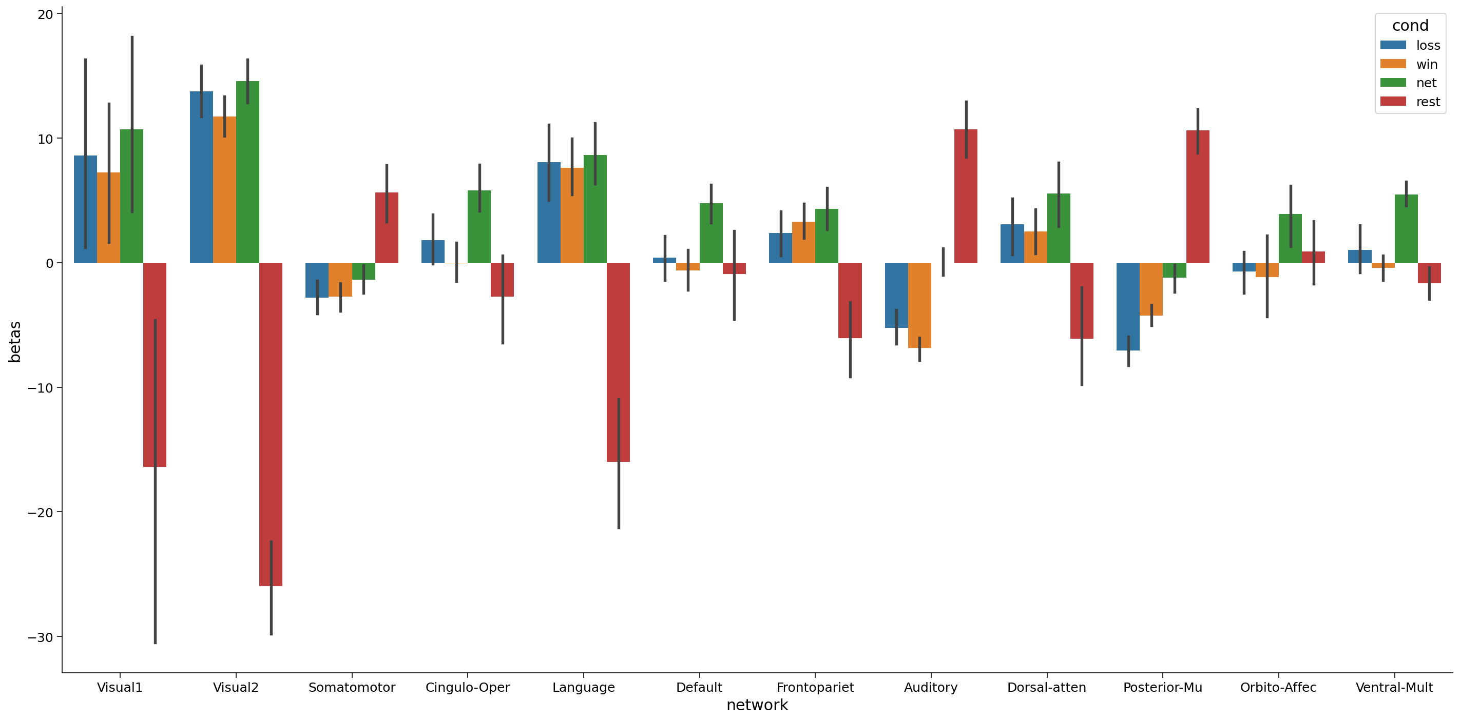
Remember that we have 360 ROI and these ROIs become 12 networks, let’s add the network component:

# plot the mean beta based on the network and compare with 4 conditions
df_beta_2  = pd.DataFrame({'betas'  : np.hstack((betas_avg_sub_run_los[0,:], betas_avg_sub_run_win[0,:], betas_avg_sub_run_net[0,:], betas_avg_sub_run_res[0,:])),
                   'cond'   : np.hstack((['loss']*360, ['win']*360, ['net']*360, ['rest']*360)),
                   'network': np.hstack((region_info['network'], region_info['network'], region_info['network'], region_info['network'])),
                   'name'   : np.hstack((region_info['name'], region_info['name'], region_info['name'], region_info['name'])),
                   'hemi'   : np.hstack((region_info['hemi'], region_info['hemi'], region_info['hemi'], region_info['hemi']))
                  })

fig, (ax1)= plt.subplots(1,1, figsize = (20,10))
sns.barplot(x='network', y='betas', data=df_beta_2 , hue='cond',ax=ax1)
#sns.barplot(x='network', y='betas', data=df_beta_2 , hue='hemi',ax=ax2)

R value with network:

# plot the mean r based on the network and compare with 4 conditions
df_r = pd.DataFrame({'r'  : np.hstack((r_avg_sub_run_los[0,:], r_avg_sub_run_win[0,:], r_avg_sub_run_net[0,:], r_avg_sub_run_res[0,:])),
                   'cond'   : np.hstack((['loss']*360, ['win']*360, ['net']*360, ['rest']*360)),
                   'network': np.hstack((region_info['network'], region_info['network'], region_info['network'], region_info['network'])),
                   'name'   : np.hstack((region_info['name'], region_info['name'], region_info['name'], region_info['name'])),
                   'hemi'   : np.hstack((region_info['hemi'], region_info['hemi'], region_info['hemi'], region_info['hemi']))
                  })

fig, (ax1)= plt.subplots(1,1, figsize = (20,10))
sns.barplot(x='network', y='r', data=df_r, hue='cond',ax=ax1)
#sns.barplot(x='network', y='r', data=df_r, hue='hemi',ax=ax2)

Now, let’s make a group contrast with beta and r value so we can really know the brain activity on different condition:

def average_frames(be, evs, experiment, cond):
    idx = EXPERIMENTS[experiment]['cond'].index(cond)
    return np.mean(np.concatenate([np.mean(data[:,evs[idx][i]],axis=1,keepdims=True) for i in range(len(evs[idx]))],axis=-1),axis=1)

loss_activity = average_frames(data, evs, my_exp, 'loss')
win_activity = average_frames(data, evs, my_exp, 'win')


#change the data structure and calculate the contrast map to fit in the brain image
loss_beta = betas_avg_sub_run_los[0,:]
win_beta = betas_avg_sub_run_win[0,:]

contrast_beta    = loss_beta -  win_beta  # difference between loss and win in avewrage beta

los_r = r_avg_sub_run_los.T
win_r = r_avg_sub_run_win.T

# contrast_r    = los_r - win_r  # difference between left and right hand movement
contrast_r    = win_r - los_r

Create group contrast map:

group_contrast = 0
for s in subjects:
  for r in [0,1]:
    data = load_single_timeseries(subject=s,experiment=my_exp,run=r,remove_mean=True)
    evs = load_evs(subject=s, experiment=my_exp,run=r)

    loss_activity = average_frames(data, evs, my_exp, 'loss')
    win_activity = average_frames(data, evs, my_exp, 'win')

    contrast    = loss_activity-win_activity
    group_contrast        += contrast

group_contrast /= (len(subjects)*2)  # remember: 2 sessions per subject

Finally, let’s plot the brain:

# This uses the nilearn package
!pip install nilearn --quiet
from nilearn import plotting, datasets

# loading the atlas
fname = f"{HCP_DIR}/atlas.npz"
if not os.path.exists(fname):
  !wget -qO $fname https://osf.io/j5kuc/download
with np.load(fname) as dobj:
  atlas = dict(**dobj)

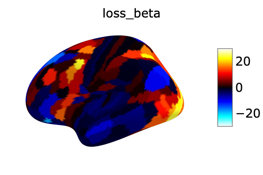
los_beta:

fsaverage = datasets.fetch_surf_fsaverage()
surf_contrast = betas_avg_sub_run_los[0,:][atlas["labels_L"]]
plotting.view_surf(fsaverage['infl_left'],
                   surf_contrast,
                   vmax=30,title='loss_beta')

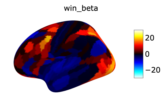
win_beta:

fsaverage = datasets.fetch_surf_fsaverage()
surf_contrast = betas_avg_sub_run_win[0,:][atlas["labels_L"]]
plotting.view_surf(fsaverage['infl_left'],
                   surf_contrast,
                   vmax=30,title='win_beta')

net_beta:

fsaverage = datasets.fetch_surf_fsaverage()
surf_contrast = betas_avg_sub_run_net[0,:][atlas["labels_L"]]
plotting.view_surf(fsaverage['infl_left'],
                   surf_contrast,
                   vmax=30,title='neutral_beta')

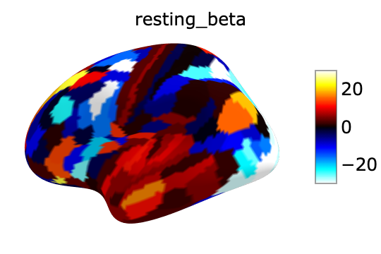
res_beta:

fsaverage = datasets.fetch_surf_fsaverage()
surf_contrast = betas_avg_sub_run_res[0,:][atlas["labels_L"]]
plotting.view_surf(fsaverage['infl_left'],
                   surf_contrast,
                   vmax=30,title='resting_beta')

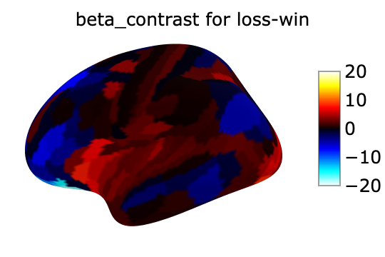
let’s see the group contast,beta_contrast:

fsaverage = datasets.fetch_surf_fsaverage()
surf_contrast = contrast_beta[atlas["labels_L"]]
plotting.view_surf(fsaverage['infl_left'],
                   surf_contrast,
                   vmax=20,title='beta_contrast for loss-win')

Congratulations! you made it. It’s time to take a break and have a cup of coffee.